Motivation
There are many software solutions that will allow you to make a map. Some of them are free and open source (e.g. GRASS) or not (e.g. ArcGIS). The argument between R and something that isn't free is pretty self explanatory, but why would we want to do our GIS tasks in R over something else like GRASS that was designed for this purpose? My usual answer to that is that I prefer a nice workflow all in R, I like the continuity. I also like leveraging my R programming know-how (e.g. data manipulation, loops, etc) to do complex and/or repeated operations that might take me longer to click through or learn how to automate in some other program. Really, you just need to find the right tool for the job, sometimes that will be R, other times it will be a dedicated GIS program. Also, R and GRASS can interact providing an intermediate solution. All that being said, it helps to know what R can do when you're choosing your tool.
Load the required packages
(also install.packages() if necessary)
library(maptools)
library(rgdal)
plus these packages if you want to go through the examples at the bottom
library(raster)
library(maps)
library(mapdata)
library(ggmap)
library(marmap)
library(lattice)
Getting your data off your GPS
If your GPS can export to .gpx format, you can read the file directly as lines (i.e. tracks), points (i.e. track_points), and a few other formats you can find in the help for readOGR. To download and example .gpx, click here
run <- readOGR(dsn="run.gpx",layer="tracks")
plot(run)

run <- readOGR(dsn="run.gpx",layer="track_points")
plot(run)
If your GPS cannot save in .gpx format, you will have to resort to GPSBabel to convert your file(s) from the proprietary file format to .gpx. Interestingly, to streamline your workflow and make your work reproducible, R can interact with GPSBabel directly through the readGPS() function which is in the maptools package
Getting a base map
There are a few ways to get this type of thing in R, I'll cover many of these in a future lesson, for now let's just use a simple world map from the maptools package:
data(wrld_simpl)
Let's plot that to see what we have
plot(wrld_simpl)
Or we can 'zoom in' on a particular spot if we provide limits
xlim=c(-130,-60)
ylim=c(45,80)
plot(wrld_simpl,xlim=xlim,ylim=ylim)
We can also give it some color
plot(wrld_simpl,xlim=xlim,ylim=ylim,col='olivedrab3',bg='lightblue')
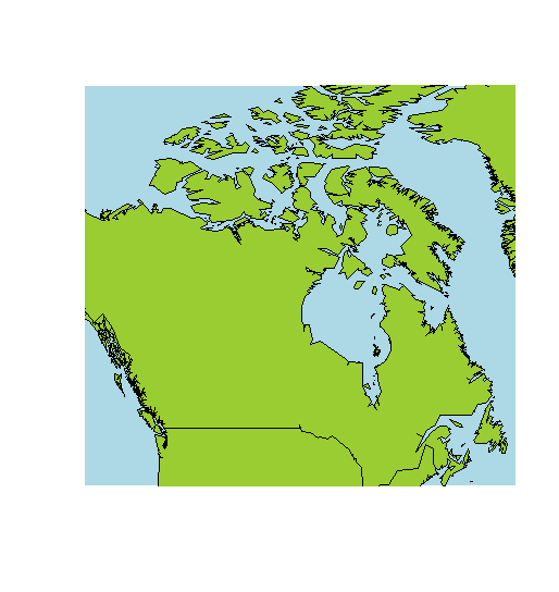
I know, the map projection is not awesome, we're going to cover that in another future lesson.
Challenge problem 1
Can you zoom in to your home town?
Exporting and importing
Now that we know how to get a super basic map in R, let's look at how we can export and import data. This will write an ArcGIS compatible shapefile, writeOGR() will actually write to many different formats you just need to find the correct driver
writeOGR(wrld_simpl,dsn=getwd(), layer = "world_test", driver = "ESRI Shapefile", overwrite_layer = TRUE)
Now we could open world_test.shp in ArcGIS, but we can also import shapefiles back into R, let's use that same file
world_shp <- readOGR(dsn = getwd(),layer = "world_test")
plot(world_shp)
Spatial data types in R
Vector based (points, lines, and polygons)
creating spatial data from scratch in R seems a little convoluted to me, but once you understand the pattern, it gets easier
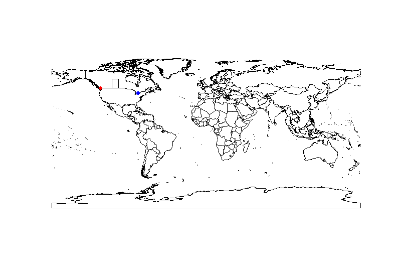
SpatialPointsDataFrame
let's plot points on Simon Fraser University and University of Toronto
coords <- matrix(c(-122.92,-79.4, 49.277,43.66),ncol=2)
coords <- coordinates(coords)
spoints <- SpatialPoints(coords)
df <- data.frame(location=c("SFU","UofT"))
spointsdf <- SpatialPointsDataFrame(spoints,df)
plot(spointsdf,add=T,col=c('red','blue'),pch=16)

SpatialLinesDataFrame
let's plot the borders of the province of Saskatchewan because they're easy to draw (but not to spell!)
coords <- matrix(c(-110,-102,-102,-110,-110,60,60,49,49,60),ncol=2)
l <- Line(coords)
ls <- Lines(list(l),ID="1")
sls <- SpatialLines(list(ls))
df <- data.frame(province="Saskatchewan")
sldf <- SpatialLinesDataFrame(sls,df)
plot(sldf,add=T,col='black')
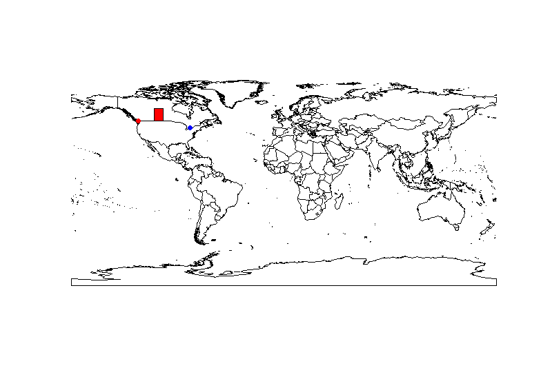
SpatialPolygonsDataFrame
let's plot the province of Saskatchewan because it's easy to draw (but not to spell!)
coords <- matrix(c(-110,-102,-102,-110,-110,60,60,49,49,60),ncol=2)
p <- Polygon(coords)
ps <- Polygons(list(p),ID="1")
sps <- SpatialPolygons(list(ps))
df <- data.frame(province="Saskatchewan")
spdf <- SpatialPolygonsDataFrame(sps,df)
plot(spdf,add=T,col='red')
Challenge problem 2
Can you plot a point on your home town?
Making nicer maps
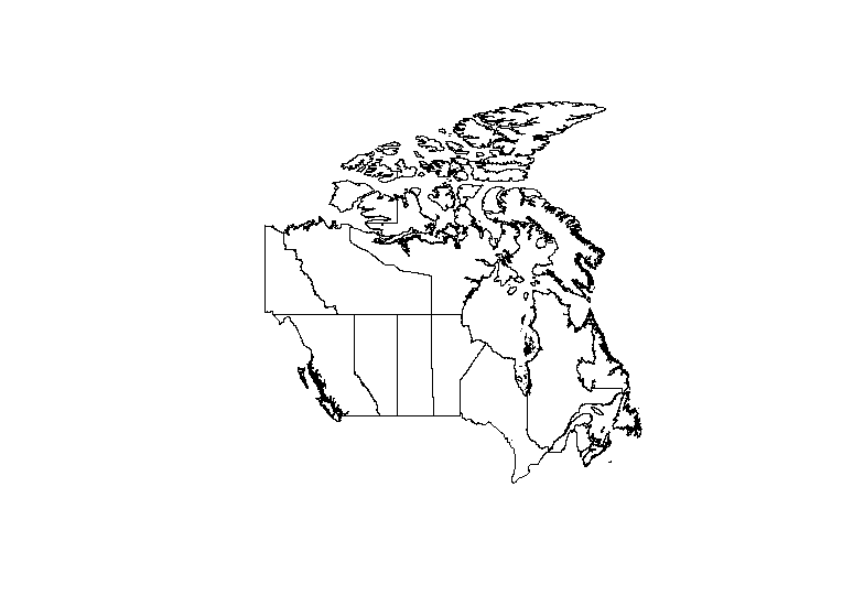
The raster package for basic maps that interact well with spatial objects we used above, unlike many other packages, this method 'plays nice' with other spatial object from the sp package and can be use proper projections etc.
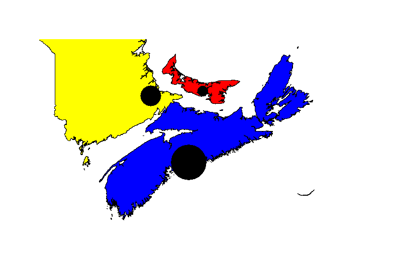
We can download polygons for Canada from GADM (amongst other sources) with the country code "CAN", and level=1 indicates provinces, 0 would be the whole country.
Canada <- getData('GADM', country="CAN", level=1)
plot(Canada)
We can manipulate this SpatialPolygonDataFrame by looking at what is inside its dataframe
Canada
We can see that the names of the provinces are in Canada$NAME_1, so lets use that to extract provinces
NS <- Canada[Canada$NAME_1=="Nova Scotia",]
plot(NS,col="blue")

NB <- Canada[Canada$NAME_1=="New Brunswick",]
plot(NB,col="yellow",add=TRUE)

PEI <- Canada[Canada$NAME_1=="Prince Edward Island",]
plot(PEI,col="red",add=TRUE)
let's plot points in Moncton, Halifax and Charlottetown
coords <- matrix(cbind(lon=c(-64.77,-63.57,-63.14),lat=c(46.13,44.65,46.24)),ncol=2)
coords <- coordinates(coords)
spoints <- SpatialPoints(coords)
df <- data.frame(location=c("Moncton","Halifax","Charlottetown"),pop=c(138644,390095,34562))
spointsdf <- SpatialPointsDataFrame(spoints,df)
scalefactor <- sqrt(spointsdf$pop)/sqrt(max(spointsdf$pop))
plot(spointsdf,add=TRUE,col='black',pch=16,cex=scalefactor*10)
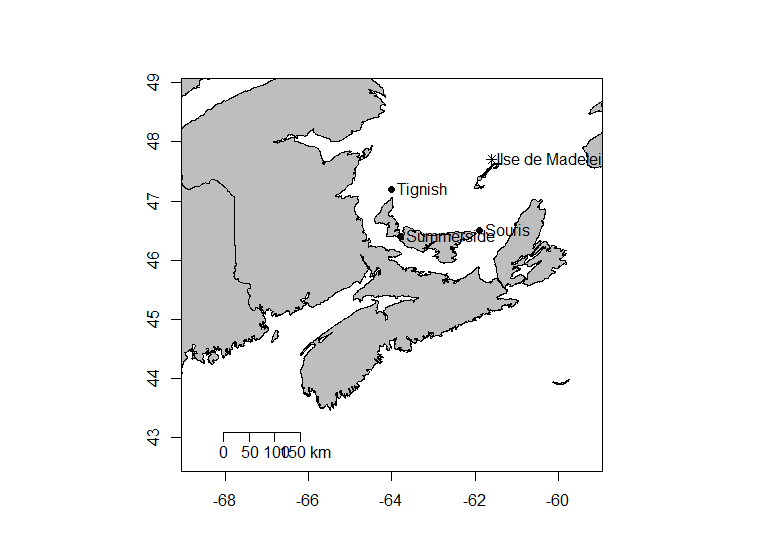
The maps and mapdata packages for basic maps:
Coordinates which highlight the scale of the map
Lat.lim=c(42.5,49)
Long.lim=c(-69,-59)
Locations of interest - these examples correspond to the tips of PEI and the provinces best city####
Site.Longs=c(-61.9,-64,-63.8)
Site.Lats=c(46.5,47.2,46.4)
Site.Names=c("Souris","Tignish","Summerside")
Make the map. Here you can play with the fill colour (now grey) and a few other tweaks
map("worldHires", xlim=Long.lim, ylim=Lat.lim, col="grey", fill=TRUE, resolution=0);map.axes();
map.scale(ratio=FALSE) # do you want a scale?

points(Site.Longs,  Site.Lats,pch=19) #Add points if you have data in Site.Longs and Site.lats
points(-61.6,47.7,pch = 8 ) # this will add point a single point (*) to the Maggies
text(Site.Longs,Site.Lats,labels=Site.Names,pos=4, offset=0.3) # add labels
text(-61.6,47.7,labels="Ilse de Madeleine",pos=4, offset=0.3) # add label to an individual plot
Challenge problem 3
Can you label your home town?
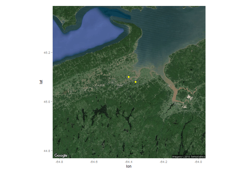
The ggmap package for Google Maps:
This package is great particularly if you are familiar with the ggplot2 plotting grammar. You may also come across the RgoogleMaps package, but I do not recommend using it because it seems to have a grammar unique to that package (i.e. not compatible with base plotting or ggplot2) and has strange scaling behaviour.
google <- get_map(location = c(-64.4,45.08), zoom = 10, maptype = "satellite")
p <- ggmap(google)
p + geom_point(aes(x=c(-64.36,-64.4),y=c(45.08,45.1)),colour='yellow',size=3)
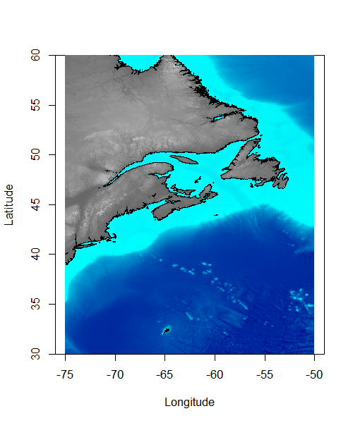
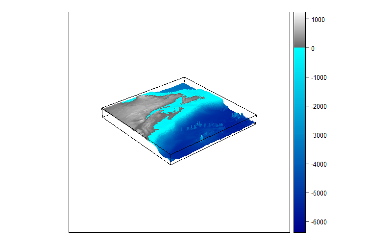
The marmap package for bathymetry:
If you're an oceanographer like myself, you will love this package! It can query and plot NOAA's bathymetry databases
Let's define some colors for sea and land
blues <- colorRampPalette(c("darkblue", "cyan"))
greys <- colorRampPalette(c(grey(0.4),grey(0.99)))
We can query to NOAA databases for bathymetry at 1 minute resultion, but lets do 10 to keep download speeds reasonable.
atl<- getNOAA.bathy(-75,-50,30,60,resolution=10)
After that's done we can plot some nice 2d and 3d plots (we will cover the details in a later study group)
plot.bathy(atl,
           image = TRUE,
           land = TRUE,
           n=0,
           bpal = list(c(0, max(atl), greys(100)),
                       c(min(atl), 0, blues(100))))
wireframe(unclass(atl), drape = TRUE,
          aspect = c(1, 0.1),
          scales = list(draw=F,arrows=F),
          xlab="",ylab="",zlab="",
          at=c(min(atl)/100*(99:0),max(atl)/100*(1:99)),
          col.regions = c(blues(100),greys(100)),
          col='transparent')
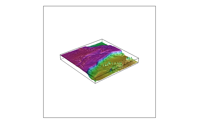
wireframe(unclass(atl), shade = TRUE,
          aspect = c(1, 0.1),
          scales = list(draw=F,arrows=F),
          xlab="",ylab="",zlab="")
Other great resources:
http://pakillo.github.io/R-GIS-tutorial/#plot